At the end of the second article of this campaign, one sentence pointed at the next project without knowing it: name collisions, linear_search_issues versus github_search_issues, survive scaling, "which suggests a format or retriever problem rather than capacity". The third article settled the format hypothesis, and the collisions survived the correction too. It closed on a finding backed by four measurements but no mechanism: cheap training installs dispositions and does not fix fine mappings. What remained was to understand why.
Here is why. It was not the format, not the retriever, not capacity. The model knows which tool is right: the information sits in its internal state, readable at 96-100% with the dumbest classifier there is. It fails to read it at generation time. The wall of 60 was not a capacity ceiling, it was a readout ceiling.
This can be measured, it can be repaired, and the repair can be confirmed. A probe on the internal states returns an unambiguous verdict, 36 measurements out of 36, significant after correction. A readout corrector, zero trained parameters, centroids and dot products, lifts the 2.9B champion from 61 to 67/82. And because that is exactly the kind of number you get by fooling yourself, we submitted it to a blind confirmation, policy and threshold frozen by a commit made before the run, on a fresh never-seen judge: +8 points, p = 0.039. All of it for about two dollars of compute, free Kaggle included. As usual, raw generations, corpora, frozen protocols and checksums are in the public bench.
The starting point is a puzzle the campaign had left open: 135 training examples aimed at seven precise confusions had fixed none of them. Errors moved around instead of disappearing. Meanwhile, general dispositions, knowing when to stay silent for instance, were learned in one epoch. Two community observations pointed the way. Smerky calls "context referral" the weakness where the information is in the state but the model cannot re-address it. And cgisky's rwkv7-state-embedding measures the same thing from the inside: a supervised probe recovers 93% of the information in the states, but the space is so anisotropic that unsupervised access collapses.
If that is the right explanation, it is testable. Extract the states at the exact moment the model must choose, and check whether a classifier separates the confused pairs there. We froze the protocol before any measurement: eight pairs the bench actually confuses (313 distinct confusion pairs collected across 56 result arms), 240 fresh queries written for the occasion and leak-filtered (Jaccard ≤ 0.20 against the public judge), a positive control that must separate, a negative control that must stay at chance, and a verdict grid written in advance. Two context regimes: the pair alone, and the bench's realistic context, forty tools in the prompt.
The verdict fits in one table. In the forty-tool context, the one where the model actually fails, behavior collapses while the state knows:
| Pair (top-40 context, raw model) | Behavior | State separability |
|---|---|---|
| All 8 pairs | 147/270 (54%) | 0.96-1.00 |
runtime_info vs model_get_info | 2/30 (7%) | 0.99 |
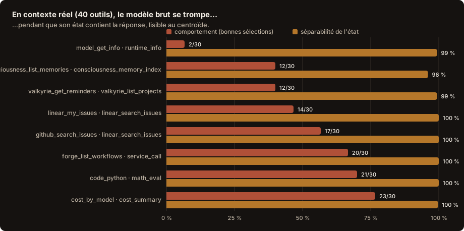
One precaution the third article taught us the hard way: a bench also measures your harness. Here the critique cancels by construction, the same prompts feed both the behavior and the states, the contrast is within-regime. And its signature is absent from the data: a wrong format shows up as unparsable outputs, and our 540 behavioral measurements contain none. Every error is a well-formed wrong tool. Judgment, not syntax.
Thirty-six pair × arm × context combinations, thirty-six significant after Bonferroni correction (1,000 permutations per cell, clean controls on both sides). And "separable" does not mean at the price of a big trained classifier: nearest-centroid on cosine is enough almost everywhere. The distinction lives in the mid-to-late layers. The hard pairs sit at chance in layers 0-9, then hit 1.00 from layer 12 on.
So the 135 examples never stood a chance: they were treating a healthy organ. Representation was never the problem. Readout is.
Two side findings are worth recording. The valkyrie_remove_subtask → valkyrie_delete_subtask "confusion" is not one: the second tool does not exist in the catalogue. It is a name hallucination, a distinct phenomenon. And the tuned state, when shown a two-tool context instead of forty, does not answer: it continues the catalogue, generating a plausible entry from the right namespace. Inadvertent proof that the state carries namespace → name associations.
If the information is in the state and centroid-readable, then a readout corrector costs next to nothing: one centroid per tool, computed once from the existing training data (231 tools × 8 queries, no new data), and at decision time, a dot product between the prefill state and the shortlist candidates.
One technical detail conditions everything else, and it illustrates the anisotropy cgisky measured: centroids learned in one context regime transfer to another at only 76%. Centering each distribution by its own mean brings that back to 95%, and subtracting the corpus mean alone does not (73%). The context's shared direction crushes the fine geometry; remove it and the signal reappears. This is what makes it possible to learn the centroids in short context, ten times cheaper.
That leaves the policy. The naive version, where the probe always chooses, fails instructively: it destroys abstention (16/17 → 1/17). A "none of these tools" centroid does not model abstention, and the model already knows very well when to stay silent, it was the first thing state-tuning taught it. Hence an asymmetric policy that follows from the failure mode: never override an abstention, only correct tool → tool, and only when the probe is clearly more confident than the generation, with a cosine margin.
| Policy (2.9B champion, public judge) | Score |
|---|---|
| Free generation (baseline, exact replication of the published 61/82) | 61/82 |
| Probe alone (selector) | 50/82 |
| Tool → tool corrector | 65-67/82 across margins, 67 at the best setting |
The plateau is the important part: 65 to 67 across the whole margin curve, zero margin included. The gain does not depend on fine tuning a threshold. Six points over the champion, without one trained parameter, with abstention (16/17) and arguments (18/22) preserved.
A +6 obtained by picking the policy and threshold on the very judge that measures it is not worth much, it is precisely the kind of result that evaporates on replication. And our 82-case judge has been public since late July: any future-wave verdict required a fresh instrument. So we did what the literature recommends and almost nobody does, a pre-registered confirmation.
Eighty-two new cases, same distribution as the public judge, each case mechanically validated against the catalogue's real schemas, leak-checked against everything that exists (public judge, training data, probe corpora), retriever recall verified at 65/65. Then a pre-registration document, committed before the run: tool → tool policy, margin 0.02, decision layer, centroids reused as-is with their checksums, confirmation criterion (Δ ≥ +3 and McNemar p < 0.05), a single scoring allowed. The measurement kernel verifies the pre-registration checksums itself before touching the GPU.
The result, in one pass:
| Confirmation judge (private, never seen) | free | corrected |
|---|---|---|
| Total | 48/82 | 56/82 |
| Simple selection | 13/18 | 17/18 |
| Arguments | 15/22 | 18/22 |
| Abstention (untouched by construction) | 7/17 | 7/17 |
Δ = +8, ten cases won against two degraded, exact McNemar p = 0.039. Criterion met. The effect replicates on queries in a different style, written by a different hand, and it grows. One unexpected detail: arguments gain three points, although the corrector only touches the tool name. Selecting the right tool makes the right arguments follow.
This confirmation judge stays private, and that is the price of its validity: a published judge is a contaminated judge for any future measurement. Ours has served once, it is burned as a confirmation instrument, a v3 will take its role. Skeptics get something better than a file to read: the full protocol is replayable, and the next round's pre-registration can happen under their eyes.
The second article ended on the 7.2B at 69/82. The composition question is unavoidable: does the readout corrector still help a bigger model? The answer comes in three parts, each qualifying the others.
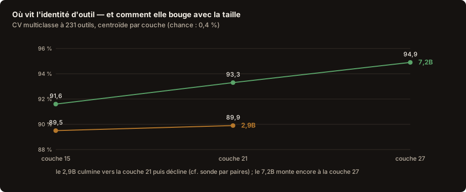
First, the probe: the internal signal improves with scale. Same corpus, same procedure, and the centroid classifier's error is halved between 2.9B and 7.2B:
| Multiclass CV, 231 tools | 2.9B | 7.2B |
|---|---|---|
| Layer 15 | 89.5% | 91.6% |
| Layer 21 | 89.9% | 93.3% |
| Layer 27 | — | 94.9% |
And the information migrates deeper: at 2.9B the profile peaks around layer 21 then declines; at 7.2B it is still rising at layer 27. Scale does not just improve the geometry, it reorganizes it.
Second, the corrector: the gain shrinks. Baseline replicated exactly (69/82, per-category profile identical to the published number), then the useful surprise: the policy calibrated on the 2.9B, applied as-is, degrades the 7.2B (67/82). A model that errs less makes low-margin corrections net-negative; a stricter margin is needed to get back into positive territory. 71/82 at the best setting, a number we label exploratory until a pre-registered v3 judge confirms it. Nothing exponential here, quite the opposite: +6 at 2.9B, +2 at 7.2B, the arithmetic of a ceiling drawing closer, with fewer errors left to harvest.
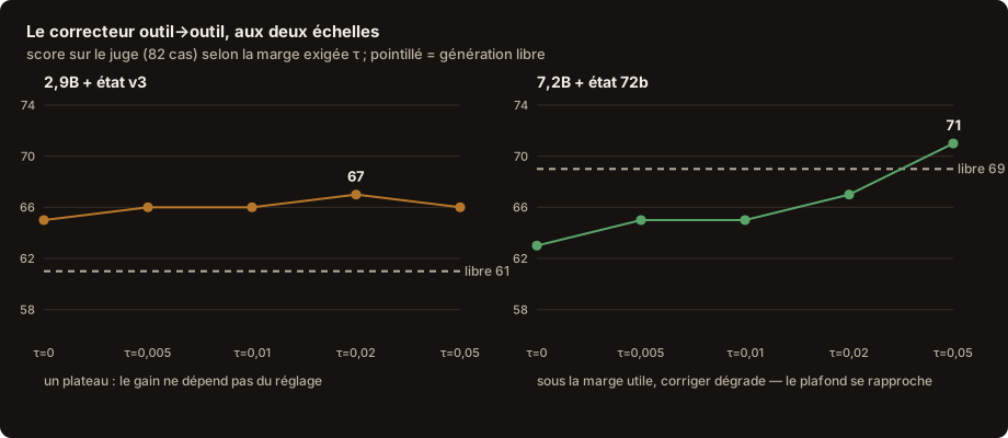
Third, composing the three facts, the signal grows, readout does not follow on its own, the corrector's harvest shrinks, gives this article's practical conclusion: the readout corrector is a small-model equalizer. The corrected 2.9B (67) lands two points from the raw state-tuned 7.2B (69), at 2.5× fewer parameters and a 150 MB artifact. Where compute is scarcest, assisted readout pays the most. That is exactly the distribution you want if you run your models locally.
A p of 0.039 on 82 cases is significant, not crushing: ten against two on the discordant cases. What makes us hold the result as real is convergence, four directionally consistent measurements across two judges and two scales, one of them blind and pre-registered. Not any single number. The 7.2B's 71/82 is post-hoc and will remain so until confirmed. The centroids come from the training-data distribution; the confirmation judge, written in a different style, already tests one generalization, but not that of real user queries in messy conditions. Abstention remains the model's weak point outside its curriculum (7/17 on the confirmation judge) and the corrector does not touch it, by construction. That is the designated next project. Multi-step stays at zero, one-turn harness, as it has from the start. And all of this lives in the native runtime: GGUF carries neither the trained state nor access to internal states, so llama.cpp production does not get this today.
The corrector's marginal cost is nearly zero: the state already exists at the end of prefill, and the corrector adds one dot product against at most forty candidates. The artifact, 231 centroids of one layer, weighs 150 MB in fp32, compressible. For the interactive 2.9B, this is the second free win identified after the second article's state cache, and the two compose: the state cached after the fixed prefix is the very object the probe reads.
The building block reaches beyond tool-calling. The same state centroids, with the same per-distribution centering, are a natural candidate for routing between trained states, or for measuring behavioral drift without the noise that made our output comparisons so misleading: two generations from the same model can be near-orthogonal, but prefill states are deterministic. More on that later.
The rest of this story is the subject of a fifth article: abstention, the weak point named above, is fixed by the same method. No raw model knows when to shut up, at any scale; its state does. With, as a bonus, a failed confirmation that we publish too.
Everything is in the bench (mirror on Forgejo): probes/state-separability/ for the frozen protocol, the corpora, the raw results and the 36/36, probes/state-reranker/ for the centroid corpus, the kernels, the free and forced generations at both scales, and the full curves, including the ones that do not flatter us. The probe and the 2.9B corrector ran on free Kaggle; the 7.2B run cost one dollar of rented A40. The confirmation's pre-registration, its judge and its single scoring are timestamped by commits; the judge stays private to remain an instrument, and its construction protocol is published.
A hole in the protocol? A competing explanation? Write to us: contact@scarletwolf.ai. That is what publishing is for.
