We train RWKV models to drive the 231 real tools of our assistant Gungnir. This post documents a result we did not expect this early: after a single epoch of state-tuning, at a GPU cost of $0.53, our local 2.9-billion-parameter RNN reaches the exact same overall score as a cloud model ten times its size on our benchmark. And the result replicates byte for byte.
Everything below is verifiable: the benchmark, the tool schemas, the raw generations, the scripts and the cryptographic fingerprints of the models are published. Hostile reviewers are welcome.
An agentic assistant receives a natural-language request and must decide which tool to call. On Gungnir that means choosing among 231 functions, many of which look alike: archive versus delete a card, search email versus search the web, five variants of cost analytics. It must then fill the required arguments without inventing any. And when the user simply says thanks, the right answer is to call nothing at all.
Large cloud models do this well. Our bet is that a small recurrent model, runnable on ordinary hardware, can learn the same trade. The stakes go beyond our product: an RNN has no KV cache, its session state stays constant in size no matter how long the conversation runs, which changes the economics of serving agents locally. We had already explored this architecture family for document retrieval; here we go after the action decision itself.
We built an 82-case judge over Gungnir's real tool schemas, split across five categories: hard selection (23 near-duplicate traps, the archive-versus-delete kind), argument filling (22), simple selection (18), abstention (17 cases where no tool should be called) and multi-step (2).
Three precautions structure this judge:
The judge, the 231 tool schemas, the scripts and the raw outputs are published in the benchmark repository (link at the end), alongside Gungnir's code, which is itself open.
The target is qwen/qwen3-30b-a3b-instruct-2507, a 30-billion-parameter mixture-of-experts with a strong function-calling reputation, queried through OpenRouter in its normal mode: all 231 raw schemas in context. Score: 58/82 (70%), with perfect abstention (17/17).
Our RWKV pipeline is different, and openly so: a retriever (a 144M RWKV embedder we had fine-tuned for search) shortlists the 40 most plausible tools, measured at 100% recall on this judge, and the model chooses among them. A small model with 4,096 tokens of native context cannot swallow 31,000 tokens of schemas; retrieval is not an optimization, it is the local pipeline's condition of existence. Both systems answer the same 82 queries, each with its own scaffolding.
Along the way, the choice of starting checkpoint taught us a lesson. We measured three successive generations of RWKV-7 2.9B published by BlinkDL: the most recent one (G1h, July 2026) is significantly worse at tool selection than its predecessor (G1g, May 2026): 29/82 versus 38/82, dominated in every category, p = 0.012 in a paired test. Progress of generalist checkpoints is not monotonic on a narrow capability. Benchmark your own use case before upgrading; we nearly trained on the wrong starting point.
RWKV-7 is a recurrent network: it maintains an internal state that summarizes everything it has read. State-tuning, from the RWKV-PEFT ecosystem, trains only the initial state of each layer: 5.2M parameters out of 2.9B, 0.18% of the model, with all weights frozen. The resulting artifact is an 11 MB file that loads on top of the base model. Think of it as a learned disposition: the model starts every request already configured for the tool-calling trade.
The data: 2,623 examples built on the real schemas, including 312 abstention cases (12%). The construction is verifiable by design: for each tool, a generator produces queries that require it, and the correct call constitutes the label, validated against the schema. Every example reproduces the exact deployment format, retriever top-40 included, sibling tools side by side so the model learns the nuances.
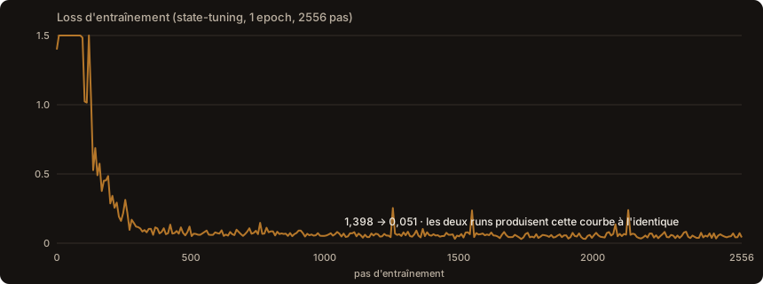
Training: 1 epoch, 2,556 steps, context 6,144, bf16, on an RTX 3090 rented at $0.22/hour. Duration: about 2 hours. Cost: $0.53. The loss goes from 1.40 to 0.05.
The full table, every model evaluated on the same 82 cases with the same scorer:
| Category (cases) | G1g base | G1g + state-tuning | Qwen3-30B (231 raw) | Qwen3-30B (+ top-40) |
|---|---|---|---|---|
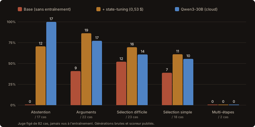
| Abstention (17) | 0 | 12 | 17 | 17 |
| Arguments (22) | 9 | 19 | 17 | 20 |
| Hard selection (23) | 12 | 16 | 14 | 17 |
| Simple selection (18) | 7 | 11 | 10 | 16 |
| Multi-step (2) | 0 | 0 | 0 | 1 |
| Total (82) | 28 (34%) | 58 (70%) | 58 (70%) | 71 (86%) |
Three readings:
The training effect is massive and targeted. From 28 to 58 solved cases. Of the 34 cases where the two versions disagree, the trained one wins 32 and loses 2 (p = 6.9×10⁻⁸, exact McNemar test). Abstention goes from 0/17 to 12/17: the model learned to stay silent. Argument filling goes from 9/22 to 19/22. These are precisely the two behaviors the dataset targeted.
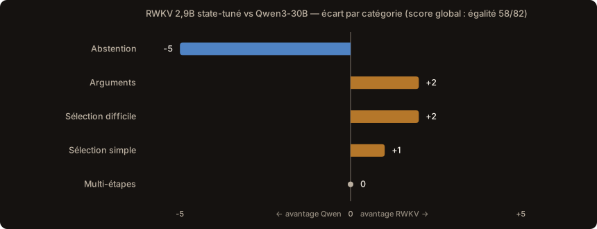
The tie with Qwen is not imitation. On the reference run, both systems score 58/82 yet agree on only 50 cases: each solves 16 cases the other misses. The trained RWKV leads the 30B on arguments, hard selection and simple selection; Qwen keeps the edge on abstention (17/17 versus 12/17).
And the target itself fluctuates. We do not. Four executions of Qwen through the API, all at temperature 0, return 57, 57, 58 and 61 out of 82: the service is not deterministic (large MoE serving rarely is). Our 58 recomputes to the character on any machine. So the parity reads like this: a deterministic score sitting at the center of the cloud model's own run-to-run band.
The format is learned, no longer enforced. The base model needed a formal grammar to produce valid JSON; trained, it no longer does: a single unparsable output out of 82, in free generation. And zero false refusals: on the 65 cases that require a call, the trained model never wrongly declined. The abstention gain did not come at the price of overcaution.
The obvious objection to the table above: our model receives a retriever-sorted top-40, Qwen navigates 231 raw schemas. Does the parity come from the model or from the shortlist? We ran the test before you could ask: same 82 cases, same top-40 per case, sent to Qwen.
Answer: Qwen + top-40 = 71/82 (86%). The shortlist is worth 13 cases to it. Two conclusions, each in its place:
We reran the entire chain on a second machine: full retraining from the base model, then re-evaluation of the 82 cases. Result: 58/82, same categories, same solved and failed cases, and the 164 generations (82 base, 82 trained) are identical character for character. Both trained checkpoints carry the same SHA-256 fingerprint.
The chain is in fact deterministic end to end: zero initial state, fixed data order, greedy decoding. This is not an average with an error bar; it is an exact point anyone can recompute. We prefer that property to a confidence interval.
A result is only useful with a sharp perimeter. Ours:
The night this was written, the second rung of the ladder returned its verdict: a LoRA (r=32, about 1% of parameters, 2 epochs on the same data, $0.90) reaches 61/82 (74%).
| Category | State (rung 1) | LoRA (rung 2) |
|---|---|---|
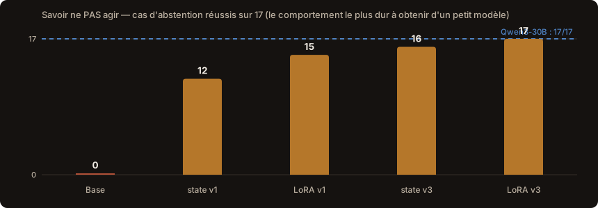
| Abstention | 12/17 | 15/17 |
| Arguments | 19/22 | 16/22 |
| Hard selection | 16/23 | 16/23 |
| Simple selection | 11/18 | 14/18 |
| Total | 58 | 61 |
Three honesty notes before applauding. One, the overall gap with the state is not statistically established (11 cases won versus 8 lost, p = 0.65): at this point, LoRA and state sit at the same level with different profiles. Two, unlike the state, LoRA starts from a random initialization: this run is not byte-reproducible, and its run-to-run variance remains unmeasured. Three, Qwen's equal-scaffold lead remains significant (p = 0.04).
What the profile tells is more interesting than the score: LoRA absorbs abstention better (15/17, only two traps left) and simple selection, but regresses on arguments (16/22 versus 19/22). More adaptation capacity does not dominate everywhere: it moves the trade-off.
The following night, three more experiments, aimed at the identified weaknesses. We added 162 purpose-built examples: 113 "actionable traps" (requests that sound like an action but that no tool covers, the precise abstention type that kept resisting) and 49 "look before you act" cases. Then we retrained both methods on this v3 data, and attempted a composition.
| Category | state v3 | LoRA v3 | combo (state v3 + LoRA v3) |
|---|---|---|---|
| Abstention | 16/17 | 17/17 | 17/17 |
| Arguments | 18/22 | 15/22 | 17/22 |
| Hard selection | 15/23 | 15/23 | 17/23 |
| Simple selection | 12/18 | 12/18 | 8/18 |
| Multi-step | 0/2 | 0/2 | 0/2 |
| Total | 61 | 59 | 59 |
Four lessons:
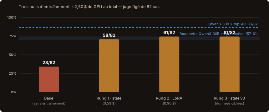
The bar remains 71/82, the 30B's score with equal scaffolding: the gap now stands at 10 cases, concentrated on selection. A replication on public tools is planned, on a fresh judge kept private until measurement.
The public benchmark repository: git.scarletwolf.cloud/kevin/rwkv-toolcaller-bench (mirror: Codeberg). It contains: the judge (82 cases), the 231 tool schemas, the evaluation and scoring scripts, the raw generations of every run (including the ones that do not flatter us), the loss curves, the pod-by-pod training recipes, and the SHA-256 fingerprints of the base model and trained states (the 11 MB files are included). The exact environment is pinned: RWKV-PEFT commit, torch and peft versions, Docker image. The cloud reference is qwen3-30b-a3b-instruct-2507 via OpenRouter.
Hardware needed to redo everything: an Ampere-or-newer GPU (bf16 is required by the RWKV-7 training kernels; Kaggle's free T4s cannot run them), about 2 hours, under a dollar.
Sovereignty and economics. An agent's requests carry the user's full working context; processing them locally removes the transfer question entirely. And an RNN serves long sessions at constant memory, where a transformer's KV cache grows with the conversation.
The 82 judge cases do not appear in the training data: 17 are hand-written, 65 were generated by a different model family with a similarity filter, and the judge was frozen before the first measurement. The very low loss (0.05) indicates strong adaptation to the format; the score on these never-seen cases measures generalization.
It is the cheapest rung of the ladder (0.2% of parameters, $0.53) and was planned as a mere plumbing test before a LoRA. It hit the target on its own. The LoRA explored further; see the rung 2 section.
That the skill is a file. Load the base model once, then hot-swap specialized states per task without duplicating the 5.6 GB of weights. That is a deployment model of its own for local agents.
The benchmark repository is public, and so is Gungnir's code. Links are in the Reproduce section. If you find a hole in the protocol, write to us; that is what publishing this is for.
